Overview of Signal Processing

It all starts with sensors.

Sensor: something that can record the environment, bring that information into the digital world. That’s when signal processing begins.

Diverse of Signals

Electromagnetism

Electromagnetic signals are generated by the movement of charged particles. They can be used to transmit information over long distances, such as in radio and television broadcasting.

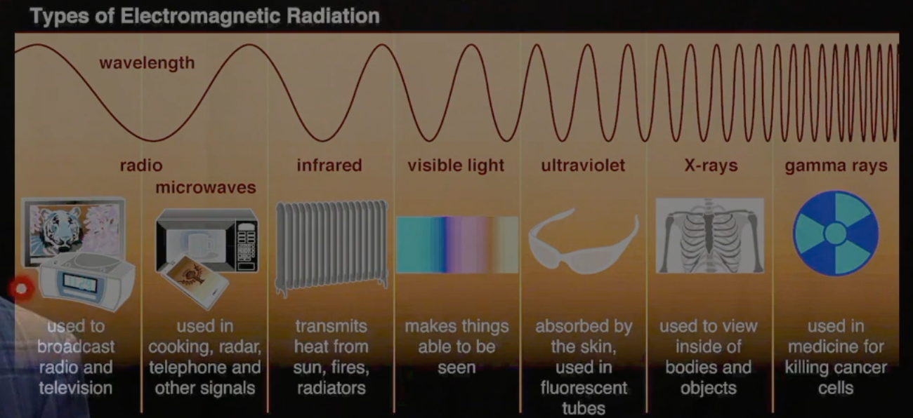
Frequency range: from a few hertz (Hz) to several gigahertz (GHz).

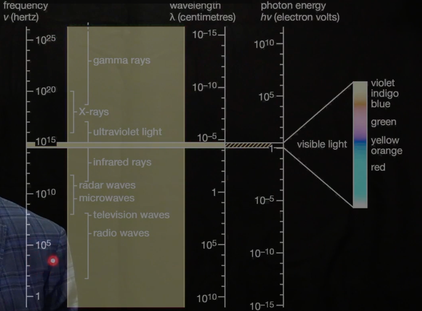
Signal-Processing-01-An-Overview-2025-11-02-22-20-38

Applications: radio, microwaves, infrared, visible light, ultraviolet, X-rays, gamma rays.

Wavelength in the range of Radio waves: used to broadcast radio and television signals.
Wavelength in the range of Microwaves: used in cooking, radar, telephone, …
Wavelength in the range of Infrared: can transmit heat from sun, fires, radiators, …
Wavelength in the range of Visible light: can make things able to be seen, the only part of the electromagnetic spectrum that can be seen by the human eyes.
Wavelength in the range of Ultraviolet: can be absorbed by the skin, used in fluorescent tubes
Wavelength in the range of X-rays: can view inside of bodies and objects, used in medical imaging
Wavelength in the range of Gamma rays: used in medicine for killing cancer cells

Signal-Processing-01-An-Overview-2025-11-02-22-22-44

Acoustics

How Acoustics are Generated: Acoustics are generated by vibrating objects

Bandwith of acoustic signals: from a few hertz (Hz) to several kilohertz (kHz).

Infrasound: below 20 Hz, used to monitor earthquakes and volcanic eruptions
Acoustic signals in the range of 20 Hz to 20 kHz: audible sound for humans, used in music, speech, and other forms of communication
Ultrasound: above 20 kHz, used in medical imaging and industrial applications

Periodic Signals

x[t] = x[t + T] or x[n] = x[n + N]

T: period in continuous-time signals
N: period in discrete-time signals

Even and Odd Signals

Even Signals: cos(t), cos[n]

x(t) = x(-t) or x[n] = x[-n]
Symmetric about the vertical axis

Odd Signals: sin(t), sin[n]

x(t) = -x(-t) or x[n] = -x[-n]
Symmetric about the origin

Basics of Signal Processing

Basic Transformations

Time Shifts: x(t) -> x(t - t0) or x[n] -> x[n - n0]

Scaling: x(t) -> x(at + b) or x[n] -> x[an + b]

|a| < 1: stretching
|a| > 1: compression

Reflection: x(t) -> x(-t) or x[n] -> x[-n]

Even and Odd Decomposition

Any signal can be decomposed into the sum of an even and an odd signal.

Even part: Xe(t) = (x(t) + x(-t)) / 2
Odd part: Xo(t) = (x(t) - x(-t)) / 2

Why?

Given any signal x(t) = x(t)/2 + x(t)/2
Then we add and subtract x(-t)/2 to complete the even and odd parts: x(t) = x(t)/2 + x(t)/2 + x(-t)/2 - x(-t)/2
Change the order: x(t) = (x(t) + x(-t))/2 + (x(t) - x(-t))/2
Label the two parts: x(t) = Xe(t) + Xo(t) where Xe(t) is even and Xo(t) is odd

Exponential Signals

Why Exponential Signals are Important?

Many signals can be represented as a sum of exponential signals (Fourier Series, Fourier Transform, Laplace Transform, Z-Transform)

Consider a simple linear dynamical system characterized by the equation:

What is the linear dynamical system: a mathematical model used to describe how a system evolves over time according to linear rules.
- Discrete-Time Linear Dynamical System: the system’s state changes at discrete time intervals.
  - x[n+1] = A * x[n] + B * u[n] where A is the state transition matrix, the matrix describing how the system evolves, , B is the input influence matrix
- Continuous-Time Linear Dynamical System: The change rate of the state depends linearly on the current state.
  - dx(t)/dt = A * x(t) + B * u(t)

Consider the most basic case on continuous-time linear dynamical system:

dx(t)/dt = A * x(t) where B = 0

To solve this, we assume an ansatz (a trial solution) in the form of an exponential signal:

x(t) = v * e^(λt) where v is a constant vector and λ is a scalar
Why exponential ansatz works? It converts a differential equation into linear algebra.

First, we assume x(t) = v * e^(λt), that means we assume the state evolves exponentially over time and in the direction of vector v.

so x(t) can be expressed by v and λ

Then we substitute into the differential equation, and found it becomes a linear algebra problem at the end.

That means solve a dx/dt problem is equivalent to solve a Av = λv problem.

$$
x(t) = v e^{\lambda t}\ \ \text{assumption}\

\frac{dx(t)}{dt} = \lambda v e^{\lambda t}\ \ \text{Differentiation}\

A x(t) = A v e^{\lambda t}\ \ \text{Right-hand side}\

\text{Equating both sides:}\ \ \lambda v e^{\lambda t} = A v e^{\lambda t}\

\text{Dividing both sides by } e^{\lambda t} \text{ (non-zero):}\ \ \lambda v = A v\
$$

Exponential signals have unique mathematical properties that make them easier to analyze and manipulate.

Notice not all the solution forms come in the form of an exponential, this is really critical for us when we think about linear systems, you should think about exponential solutions are the canonical solutions.

The eigenvalue problem is sort of the canonical representation of the solution

Imaginary Exponential Signals

Case 1: alpha is a real number, then the solution is a real exponential signal, which can represent growth or decay of the signal.

Those signals are not that interesting, because they are not oscillatory, they are just growing to infinity or decaying to zero.
What we really want is a signal that persists over time, that is where imaginary exponential signals come in.

$$
x(t) = e^{\pm i\omega t} = \cos(\omega t) \pm i \sin(\omega t) \ \ \text{Euler’s formula}
$$

Case 2: alpha is an imaginary number, then the solution is an imaginary exponential signal, which can represent oscillations in the signal.

Based on Euler’s formula, they are nothing more than cosines and sines
And based on the properties, those signals are defined in terms of their frequency \omega,
These signals are periodic. $$e^{i\omega t} = e^{i\omega (t + T)} = e^{i\omega t} \cdot e^{i\omega T}$$
Periodicity condition: $$e^{i\omega T} = 1 \Rightarrow \omega T = 2\pi k, k \in \mathbb{Z}$$ so the period T is related to the frequency \omega by T = 2\pi k / \omega
[ ] How can I understand the imaginary Exponential signals?

Prerequisites for Beginners

Electromagnetism Basics

Where is Electromagnetism from: the interaction between electric charges and magnetic field and the forces associated with them.

Four Foundamental Interactions in Nature: Gravitational, Electromagnetic, Strong Nuclear, Weak Nuclear.
Electromagnetism = Electricity + Magnetism

What is Electricity?: You should familiar with Static Electricity, which is created by rubbing certain materials

How Electricity is created?: the transition of electric charges (electrons).

What is electric field?: it is a abstract concept to describe the force that a charged particle would experience in the presence of other charged particles.

What is Magnetism?: it is a natural physical phenomenon, used to describe the forces

How magnetism is created?: by moving electric charges.

How magnet works:
- Electron spins create tiny magnetic fields
- When many electrons spin in the same direction, their magnetic fields combine to create a larger magnetic field
- But most materials have electrons spinning in different directions, so their magnetic fields cancel each other out

So till here, we know that moving electric charges create magnetic fields, and now let’s see how magnetic fields can create electric fields.

the motion of magnetic field will disturb the electric field, push the force on the electrons
Applications: wind turbines, nuclear power plants, telephones(motion signal to electric signal)

Electromagnetic Waves: Together, the change in electric field disturbs the magnetic field, and the change in magnetic field in turn disturbs the electric field, this kind of alternation allows electromagnetic energy to propagate in the form of waves.

Electromagnetic Spectrum: EM waves have different wavelengths and frequencies, forming the electromagnetic spectrum.

Key properties of Electromagnetic Waves:

Amplitude: the height of the wave, related to the energy of the wave
Phase: the position of the wave at a specific point in time
Wavelength: the distance between two consecutive peaks or valleys of the wave
Frequency: the number of waves that pass a specific point in one second
Speed: can be calculated by multiplying the wavelength and frequency
- Note: In a vacuum, all electromagnetic waves travel at the speed of light, which is approximately 3 x 10^8 meters per second. So that the wave with a large frequency will have a short wavelength, and vice versa.

Why Electromagnetic Waves have different types?: because the moving charges have different frequencies. So they will have different wavelengths, and then have different abilities

Signal-Processing-01-An-Overview-2025-11-03-21-43-52

How Electromagnetic Waves Carry Digital Data: digital modulation, to change one of the wave properties (amplitude, frequency, phase) to encode information.

Amplitude Modulation (AM): changing the amplitude of the wave to represent data, (0 and 1)
…

Eigenvalues and Eigenvectors

Eigenvectors are special vectors that only change by a scalar factor when a linear transformation (A) is applied to them. The scalar factor is called the eigenvalue.

For one specific linear transformation A, there can be multiple eigenvalues and eigenvectors.
Example: For matrix A = [[4, 1], [2, 3]], the eigenvalues are 5 and 2, with corresponding eigenvectors [1, 1] and [-1, 1].

But why they are important? What’s the point of finding eigenvalues and eigenvectors? Why bother?

They help us understand the behavior of rotations: the eigenvectors indicate the axes of rotation
In signal processing, they enable efficient analysis of linear systems and transformations.

Application 1: Fibonacci Sequence

Resources

Signal Processing

Introduction to Signal Processing: An Overview (Lecture 1)

Electromagnetism

Basic of Signal Processing

Decomposing functions into an odd and even function

Overview of Signal Processing

Diverse of Signals

Electromagnetism

Acoustics

Periodic Signals

Even and Odd Signals

Basics of Signal Processing

Basic Transformations

Even and Odd Decomposition

Exponential Signals

Why Exponential Signals are Important?

Imaginary Exponential Signals

Prerequisites for Beginners

Electromagnetism Basics

Eigenvalues and Eigenvectors

Resources

Questions